For my third dataset I picked what looked like a more complex dataset with a classification task. The Internet Ads Dataset has 1558 features and a fair amount of missing data, and the goal was to classify a given online image as either an advertisement or a non-advertisement. It turned out that the vast majority of the 1558 features were simply binary flags for words/phrases that occurred in the url or alt-text or caption of the image, and with 3 real-valued features representing the dimensions of the image.
Still, this dataset offered some new challenges and I ended up learning a few things.

I started with running the dataset through some of my basic ML algorithms, with good results, and finally ended up writing a simple Neural Network as well to work with the data. In the end (spoiler alert!) I realized that using a neural network was overkill and unnecessary for this dataset – but luckily I only realized this after having already gained some useful experience from the effort.

 

 

The Data

Three of the features were real-valued: the height, width and ratio of the image. Up to 28% of the data had missing values for these features.

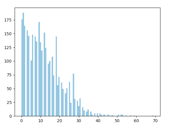
The rest of the features were binary, indicating the presence of certain words/phrases in the urls, captions and alt-text. E.g. “labyrinth“, “images+buttons“, “tvgen.com“, “http://ads.switchboard.com/“, “romancebooks“, “direct“, “unc.edu“, “sw“, “sv“, “gg“, “netscape“, “products“, “chat“, “news“, “home+page“, etc. Many such features could be active for a given input, as seen on the histogram on the right.

 

Implementation notes

• Missing Data: To handle the missing values for the 3 image dimension features, I tried two approaches:
  (a) simply dropping the rows that contained missing data (but this was unsatisfying since 28% of the data had missing values), and
  (b) computing the means of those features over the training set, and using those means to fill corresponding missing values in the training set as well as validation and test sets.
  • Wrong way to do it: Initially I made the horrible mistake of filling the missing values with the per-class means. The problem with doing this is that it inserts  knowledge about the output classification into the input features, which would obviously make things easier for the model, especially if we do that for the validation and test sets.
  • Further work: I would love to try implementing imputation techniques such as regression substitution and multiple imputation. I suspect these will better model the input data and therefore fill better values for the missing data.
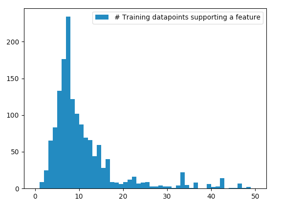
• Representative training set: I initially struggled to figure out how to bring together a training set that was representative of each of the features. Seeing that some features were supported by very few datapoints, it seemed worthwhile to figure out.
  However, I now realize that doing so would violate the principle that we’re not in control of which data gets to be the training vs. the test set.

Bayes and Naive Bayes plug-in classifiers

Of the classifiers I tried for this dataset, these are ones I struggled the most with. I eventually gave up on the Bayes classifier (see implementation notes below) but for the Naive Bayes classifier, with a small hack, I was able to achieve a 94.6% test accuracy.

Implementation notes

• Zero determinant: The main issue with Bayes and Naive classifiers was that the matrix determinant ended up being 0, which prevented any useful analysis. The 0 determinant makes sense though, because when modeling the data in a class-specific Gaussian, a lot of the features (axes) may have a non-varying value (e.g. exactly 0) for all training data points, i.e. a Gaussian with zero variance along that axis, therefore causing a zero determinant.
•  Forcing a non-zero variance: I tried shifting the variance from 0 by adding a tiny constant, and I also tried adding small random gaussian noise. This appears to solve the problem for Naive Bayes but the issue persists for Bayes. Perhaps the multiplicative effect of small axis variances ends up forcing the determinant to zero anyway.
• Further work: Although I gave up on this for now, I wonder if there is still some useful way to do per-class gaussian modeling while ignoring the subset of axes that are zero variance (Note that the subset would differ by class).

Perceptron

I initially neglected the Perceptron since I didn’t expect much from it but when I tried it later, I was surprised to get a good 96.2% test accuracy.

In hindsight, this should not have been surprising, since the dataset is filled with features (axes) that are binary (0 or 1 along each axis). Finding a hyperplane that neatly bisects the data in this 1558-dimensional space should be easy. It’s practically a kernelized space, like each input row was given its own orthogonal axis!

 

Logistic regression

With the logistic classifier, I was able to get a good 97.2% accuracy on the test set. This should also not be surprising, for the same reasons as with the Perceptron.

Implementation notes

• Initializing weights: I assumed it would help to initialize the weights w to a gaussian random, or to really small values (the same as with neural networks) but it made no noticeable difference. This makes sense because the problem of symmetry in neural networks has to do with weights across the hidden (logistic) units, and not across the weights feeding a single logistic unit, which will be differentiated because of the differing inputs they’re tied to.

 

SVM classifier

The linear SVM gave me a 96.75% test accuracy, around the same as Logistic and Perceptron.

For the kernel RBF SVM I was able to get a test accuracy of around 97.27%, slightly better. (This was using scikit’s kernel SVM. See notes below.)

Implementation notes

• Computing the K matrix: When training my own RBF kenerlized SVM on this dataset, my computer consistently ran out of memory. On closer inspection, this was not surprising, since my vectorized implementation for calculating the K matrix temporarily creates a 3d matrix of 3 billion elements before collapsing the 3rd dimension. I will need to find a better way to compute this matrix.

 

Neural Network

I next implemented a Neural Network (NN) to do classification on this dataset. NNs initially seemed to me to be a good choice for this dataset because of how poorly the Bayesian approaches were handling the large number of input features. I learned a lot from getting the NN to work for this dataset, even though in the end it turned out that the NN was overkill.

For a small NN with a hidden layer consisting of 20 sigmoid units and with suitable regularization, I got a 96.9% accuracy on the test set.

Implementation notes

• Early learning: Training the NN with my initial set of parameters, it appeared that the NN was learning something, since the cost (negative log likelihood) was going down. And the accuracy got to around 84%.However, I eventually realized that the NN was only “learning” to classify every input as a “non-ad” and thereby getting 84% right. This kind of thing happens when (for some reason such as saturation) the earlier layers are not yet learning anything and the output layer alone is learning.
  Moreover, I believe that the cost curve above mostly represents the large regularization cost rather than error cost.
  Eventually, with a high enough learning-rate, I was able to get better training accuracy, around 97.9%.
• Optimizing training: The NN was still very slow to learn, around 1000-2000 iterations. So I set out to optimize this training speed (which in hindsight I should’ve done at the outset.) I ignored the regularization and focused on improving the learning rate (with and without dampening) . I also kept an eye on the saturation of the sigmoid units. I was able to reduce needed iterations to much less than 200.
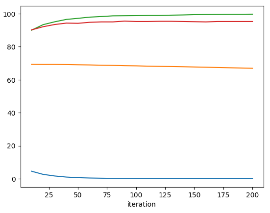
  plotting the training accuracy, the validation accuracy, the output cost and the percentage of hidden units that are saturated.
• Saturation: Note that the saturation started high and was decreasing gradually. To avoid the high saturation I initialized the weights to very small random values (-0.05 to 0.05) and saw a dramatic improvement in training speed. Playing with the learning rate also helped exhibit the effect of saturation on learning:
  The hidden layers do not contribute to learning until the saturation drops, at which point the training accuracy jumps up.
• Hidden layer size: Finally, I wanted to see the effect of hidden layer size on the output accuracy. The saturation graphs from earlier hinted that the network could still learn despite a high percentage of saturation. So I dropped the number of hidden layers from 100 to 20 and noted that the validation accuracy stayed the same. I then dropped it further to 10, then 5, 3, 2 and finally 1, and I discovered that the validation accuracy was barely affected.  At hidden layer size 1, the NN essentially acts as logistic regression, which itself was performing quite well earlier, so in hindsight this should not have been surprising…
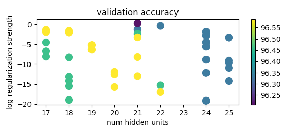
  A neural network is overkill for this dataset.
• Fine-tuning parameters: I implemented the cross validation approach of random parameter selection, which produced the following validation accuracy plot:
  from which I handpicked parameter values for testing on the test set.
• Further work: There’s a lot left to explore in Neural Networks although this dataset was too simple to go further. I hope to work on these aspects soon:
  • Batch processing
  • Dropout
  • Batch normalization