I’ve been learning Reinforcement Learning by applying it to a fun problem: Optimizing a race-car’s path along a race track. After my previous experiments with a full-state table lookup, in which I was able to get satisfactory results with the Q algorithm, I tried to see if I could achieve better results with Q(λ) or Sarsa(λ) which I suspected would solve some of the problems I was facing, especially with exploration.

Rewards and incentives

When trying to solve agent-training problems such as these, it’s natural to focus heavily on getting the agents to learn as quickly as possible, and that’s where the various algorithms and learning parameters come into play. However, a more fundamental issue needs to be addressed as well. The agent needs to be incentivized to “do the right thing”. Translating the vague idea of “the right thing” into an actual system of rewards for the agent to optimize is non-trivial and a careless approach can lead to poor results.

In my previous experiments, I stuck to a reward structure that penalized every time-step with -1, rewarded every milestone with +10 and every end-of-episode with +5000 x progress. I got reasonable results with those but the best paths discovered were never quite as optimized as I would’ve liked. It almost seemed like the agent was satisfied to reach the finish line and wasn’t giving enough seriousness to the time taken…

Dropping the progress-reward completely (to zero) notably improved the results. It turns out that the 5000 reward was overwhelming the smaller -1 time penalty in the early stages of learning; and in the later stages of learning – when the potential 5000 reward was already maxed-out and the only gains remaining would have to be made on the time-penalty – it was too late because exploration had already died out for those early stages.

On the other hand, penalizing the time-taken too much will lead to other problems, such as the agent’s preference to crash-as-quickly-as-possible. We want the algorithm to continue pursuing higher rewards, so we’re tasked with figuring out a good balance between the two incentives. In my case, introducing a small car-crash penalty of -20 seems to have done the trick.

Gamma

It might seem intuitively that gamma is a parameter that could be tweaked to train the agent faster, in the same sense that alpha or lambda or the algorithm itself can be picked to make a quick job of reinforcement learning. However, this is the wrong way to think about it.

Gamma is a parameter that directly impacts the reward scheme of the problem. Quite simply, it diminishes the importance of distant rewards as compared to that of immediate rewards. In a sense, gamma directly modifies the rewards themselves.

Results

Circular track

I seemed to get better results with Sarsa(λ) than Q(λ). The Q(λ) algorithm appeared more unstable and wavering in its final solutions.

For the circle track, Sarsa(λ) arrived at the optimal result (198 time steps) but was only slightly faster at finding it than its non-λ version. Q(λ) on the other hand did clearly worse than Q, both in speed and optimality.

Rectangular track

Similarly for the rectangular track, the Sarsas performed better (optimal solution of 202 time steps) than the Qs (best achieved 230 time steps). The λ versions of the algorithms performed slightly better than their respective simpler versions.

Giant X track

And finally for the X track, the same situation yet again: Q algorithm performed much poorer than Sarsa. Q(λ) performed poorer than Q(0). Meanwhile, Sarsa(λ) worked notably quicker than Sarsa(0) and produced slightly better results.

Implementation notes

• Smarter initialization of Q-lookup table: I considered initializing Q-table to reasonably good starting values so that it could start off on a good note and make quicker progress. However this approach was not effective, for two reasons:
  • I didn’t really know what the good values were intuitively. I might make a good guess about the effect of juncture or speed but anything beyond that (such as direction or lane) gets complicated quickly.
  • Because of the intensity of exploration that happens in the beginning, these initial values would get quickly over-written with poorly learned values anyway.
• Scoring for unfinished runs: For the purpose of cross-validation, I needed a way of scoring the models but the obvious measure of “time-taken to complete the track” would not work for models that failed to reach the finish line. So I used a score based on the average reward gained per-juncture-reached. This gave me a usable performance score.
• Using gamma instead of time-penalty: While trying to improve the path optimization of my algorithm, it occurred to me that instead of penalizing the number of time-steps taken, I could simply lower the gamma value to something less than 1, say 0.9. In theory, this would’ve incentivized the agent to get the milestone rewards sooner rather than later.
  However, gamma does its job (of diminishing future rewards) at every action step. In the case of the race-car problem, actions occur at every juncture – not at every time-step. In effect, setting gamma < 1.0 would’ve incentivized reducing the number of junctures to the finish-line, which is meaningless because that number is fixed for a given track.
• A faster eligibility rule: For forward-looking λ algorithms, it becomes necessary for a state to “receive” the effect of all future rewards. Rather than update the state value at every future step, I simply kept track of the changes until the end of the episode and made the appropriate value change a single time.
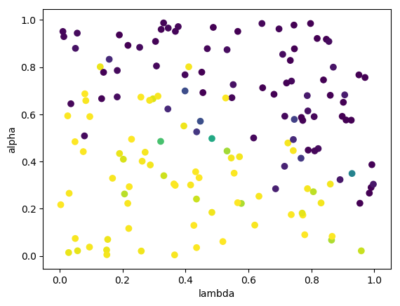
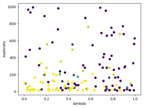
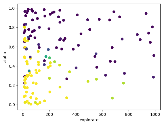
• Cross-validation: I ran cross-validation to find good parameters for alpha, lambda and explorate. I plotted 2-D graphs for each pair, for example for Q(λ):
  

  

  

  

   

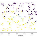
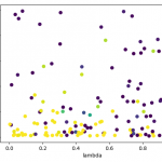
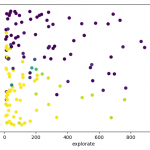
  This allowed me to pick good parameters, which I then used for learning a model, whose “best path” I then recorded.

• What does cross-validation even mean here?: In this racecar problem, although I can act as if the episodes create a “training dataset” that the algorithm learns from, I can’t act like I have a “test set” or a “validation set”. The model generated doesn’t actually have any future purpose. We simply pick the “best path” found amongst the various generated models, and that’s our answer.I believe that this quirkiness is on account of this racecar problem being fully deterministic. In the case of non-deterministic environments (e.g. a robot in real life, or an agent playing against another player), where there is no one single “best path”, cross-validation may play a more meaningful role.
• Dumping statistics to file: In order to be able to gather more data, whether through running more iterations on the same model, or running more tests of hyperparameters, I incrementally stored relevant statistics to disk, which I could later simply read and plot graphs from.
• Unstable λ runs: I noticed that the λ algorithms often had their “best paths” fluctuate quite a bit, in the end sometimes settling for a worse path than an earlier path now forgotten. On the other hand, the non-λ versions were quite stable and almost never drifted away from an existing “best path.”
  I believe this can be explained by noting that as λ grows from 0 and approaches 1, it behaves more and more like a Monte-Carlo system, which has a higher variance because all the future rewards are taken into account for every state.
• More ideas to explore:
  • Decay alpha, perhaps after the finish line has been reached. This might help the Qtable get updated quickly in the beginning and fine-tuned later.
  • Why does Q algorithm show such high variability in best-path length, and why is Sarsa notably stabler and more optimal?
  • Real-valued rewards: Due to the discretized way I have reduced this problem, there is a fair amount of accuracy that may be lost. Among these is the accuracy lost due to discretization of the time penalty. So, for example, an agent that takes 3 time steps to go from milestone A to the next milestone B is penalized with -3 regardless of whether it only just made it to B or whether it has overshot B by quite a distance already. If I were to calculate the penalty as the actual time taken, say 3.1 or 3.9, then perhaps the learning would go smoother.
    This remains to be tested, although I suspect the improvements would be small.
• Source code on github

Next steps

Having gotten these algorithms to work using the Q-lookup table, it is time to get them to work with function-approximator models such as polynomial regression and neural networks.