I had studied Support Vector Machines lightly in Prof. Ng’s ML coursera course, and then with further mathematical rigor in Prof. Paisley’s ML ColumbiaX course, but neither involved actually implementing the algorithm. It turns out that these courses never actually taught how to implement the SVM (despite giving off the impression that they had) and so what I assumed would be a straightforward python implementation ended up being quite an educational process.

Here are my notes, pitfalls and lessons learned from implementing the SVM.

Implementation notes

• Not gradient descent: I started off implementing an SVM under the false notion that once the primal problem was converted into a dual problem, the resulting “convex” function was to be solved with (essentially) a gradient-descent algorithm. (I believe I got this impression from Prof. Ng’s coursera class in which the SVM was compared very closely to Logistic Regression, the only difference seemingly being the hinge vs sigmoid loss functions (ignoring kernels for now.)) So I spent a lot of time trying to figure out how to get gradient descent to work within boundary constraints, most of my ideas revolving around using Linear algebra, but (not shockingly) I didn’t find a solution. It turns out I was trying to reinvent the wheel for a very complicated problem that has its own field of research, called numerical optimization.
  In particular, SVMs have traditionally been solved by Quadratic Programming (QP) methods (i.e. numerical optimization techniques for minimizing a quadratic function, subject to a handful of linear inequality constraints.)
  Confusingly, nowadays, there are a variety of techniques out there for solving SVMs (depending on the application, size of data, etc.) and it appears that research is ongoing. There are a couple of well-established options already (e.g. SMO), and it is usually recommended to just use an existing library (e.g. libsvm) that implements this.
• Quadratic Programming: Wondering if QP was straightforward enough for me to implement by myself, I researched more about it online. I decided it was a bit too much to take on right now but here’s the gist of how it is solved:
  Linear Programming (i.e. optimizing linear functions subject to linear constraints) is quite a bit easier to solve than QP and there are several heuristic methods (e.g. Simplex) to help find the answer quickly. Essentially, the function is evaluated at various corners located on the boundary of the solution space, until we find the one that gives the best results. As for solving QP, it turns out that a QP problem can be reduced into an LP problem plus some small hacks.
• Primal vs Dual SVM problem: Traditionally, the SVM primal optimization problem (on w) is converted to a dual problem (on alpha) and that is solved via QP. However, it turns out, it’s not absolutely necessary to follow this path. One could solve the primal problem with QP (although the dual is supposedly faster). This is especially true for non-kernelized SVMs in which w is not infinite-dimensional. Moreover, strictly speaking, it appears to be possible to do gradient descent on the primal, including with kernelized SVMs.
• Implementing SVM using QP libraries: Despite QP being the older approach (as compared to faster non-QP algorithms like SMO), this is the approach I decided to implement, for the sake of learning. The CVXOPT python library provides solvers for Quadratic Problems. I needed to translate my SVM notation into the form accepted by the library. (Confused at the time, I tried to do this for the SVM primal problem, before ultimately realizing that my dual problem was what the library required fed as the primal.) My solution ended up very similar to this blog post that explains this translation step well, although I extended it further to handle slack variables for soft-margin SVM.
• Calculating the basis w0: We can calculate w0 as described in the CSMM course material, i.e., find a non-zero alpha in the solution and for that datapoint, w0 can be easily calculated by setting to zero the inequality equation. I rounded the alphas to the fifth decimal space (because none of them were zero otherwise.) The positive alphas looked pretty huge, in the tens of thousands (which makes sense because they are not restricted by lambda, the slack parameter)
• WDBC dataset: At this point, I was able to successfully run a simple linear SVM on the WDBC dataset (which is a fully separated 2-class dataset) and also a soft-margin linear SVM on the same dataset. Soft-margin linear SVM gave an accuracy which matched that of logistic regression (around 97% test accuracy). I was further able to run SVM with an RBF kernel – the results were comparable to soft-margin linear SVM, which makes sense because the data is easy to separate into two classes.
• Calculating the basis w0 for soft-margin SVM correctly: Things started to fall apart when I tried running the soft-margin linear SVM on the Abalone dataset, which is not only a multi-class dataset, but also one with significant overlap between the classes. The results I obtained were very poor and were even worse with Hard-margin SVM (without slack variables).
  On closer inspection I noticed that w0 — far from being the same across all data-points that had alpha=0 — varied wildly in an unpredictable way. The alphas were mostly either zero or exactly lambda (aka C, the slack parameter) and if neither, then somewhere in between the two (which I initially thought was a problem but no it’s not).  I reworked the w0 calculations, taking into account mu (the legrangian parameter for the epsilon slack variables) and realized that for the w0 calculations I should focus on exactly those data-points that had both alpha=0 and mu=0. To my delight, this made everything work – all these potential w0s were equal, and the soft-margin SVM results improved dramatically. [To be honest, I still don’t fully understand why this works. In the case of hard-margin SVM, I understand that the optimization problem forces many data points to have alpha=0 (i.e. not support vectors) and can thus be ignored. But why, in the case of soft-margin SVM, does the optimal solution require some alpha and mu to be non-zero?]
  I was now able to get classification results on the Abalone dataset that were comparable to Logistic Regression.
• QP solver speed: Presumably because of the significant class overlap, the SVM (specifically the QP solver) ran much slower on the Abalone dataset than the WDBC dataset.
  Moreover, my SVM / QP algorithm runs noticeably slower than sklearn’s SVM algorithm, around 60 times slower! (This may be an issue with using the Quadratic Programming approach to SVM optimization.)
  To help speed up cross-validation, I allowed caching of Kernel matrix but this only helped a little, since the major cause of slowness was the QP library.
• Multi-class classification: In addition to the “linear” multi-class classifier I had developed earlier (which assumed a mostly linear progression of classes and the hyperplanes between them) I now implemented a one-vs-all multi-class classifier. This was not possible earlier because the “middle” class would not have been able to be surrounded by a hyperplane that was linear (say a linear Logistic or linear SVM hyperplane.) Now with a gaussian RBF kernel, this curved hyperplane would indeed be possible.
  • Update: I realized that a one-vs-one classifier would be able to handle the “linear” separation of classes, even just with linear hyperplanes dividing them, and then the “middle”ness of the middle class wouldn’t be a problem. I implemented this and got better results than my hacky solution.
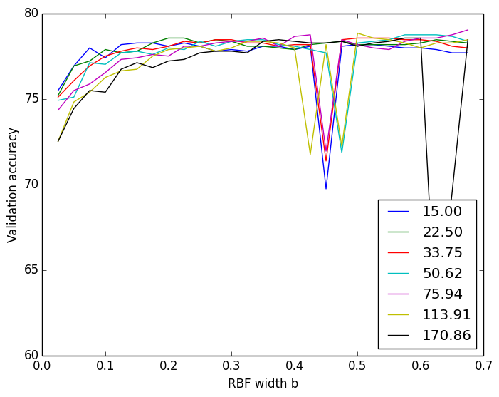
• Cross-validation and multi-class: I implemented cross-validation in order to narrow down the ideal parameters for lambda (slack parameter) and b (RBF kernel width). In order to further improve on this for multi-class classification, I performed cross-validation separately on each of the three one-vs-all classifiers, finding a dedicated ideal lambda and b for each. 
• Debugging woes: Detecting and ironing out bugs in ML algorithms can be a challenge. Here are some issues I faced:
  • It’s often not obvious whether there even is a bug. Plots and graphs are routinely wavy and spiky, and poor test accuracy may not be the fault of the algorithm. I cheated by comparing my results with those of well-known libraries, and could thus easily spot a difference in behavior. (Perhaps this is always a valid route to take, as long as we’re only reimplementing well-known algorithms (e.g. for scaling purposes), and not inventing new ones.)
  • As a further example of how bugs can slip through, I had a significant bug in which I was mistakenly testing the validation set‘s X input against the test set‘s Y output and yet I obtained a respectable 68% accuracy, only a little lower than expected.
  • Running cross-validation on SVM is the first time that my ML program has taken up hours to run to completion on my laptop. This brings with it a significant slowdown in feedback loop. I improved the logging in the code but this mostly only helps when trying to debug a known bug.
• “Overfitting” – red herring: I struggled for a long time on what seemed like an overfitting problem — i.e., the model performed well on the training set but poorly on the validation set. In fact, the validation set performed extremely poorly, and no amount of parameter tweaking seemed to improve things in any predictable way. Ultimately it turned out not to be an overfitting issue at all, instead it was a simple bug – I had normalized the training set but forgotten to normalize the validation set.
• Floating-point bugs and rounding: It was only when running the classifier hundreds of times (during cross-validation) did certain bugs rise to the surface:
  • One such bug was causing spiky results (i.e. right plot as compared to left.) 

    

    

    I found that of the data points with nonzero alpha and mu, not all were producing the same value for w0 and this was concerning. (This bug mostly showed up for classifiers with a small b width and a large lambda.) Closer investigation showed that the faulty w0′s all came from data points whose alpha or mu were quite close to zero but not exactly zero – they could be up to 1% (of lambda range) away from zero. Rounding those off to zero helped quite a bit.

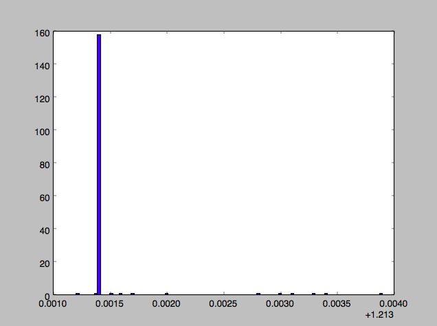
  • There continued to be a few small spikes/deviations in validation accuracies (compared to sklearn’s results). It turned out that occasionally there still remained a very few w0s in the lot that were not equal to the others, and randomly one of those w0s would get picked.
    So, I tried simply using the most common w0 value (i.e., its mode). This helped things further.
  • … but still not perfectly. From the logs, I saw that it performed poorly in those cases where all of the w0s were minutely different from each other.
    I therefore switched from taking the mode to taking the average of all the (almost identical) w0s to arrive at a final w0 to use. This finally gave me a cross-validation plot that was near-identical to sklearn’s results.
    
  • Sadly, while this worked well for the Abalone dataset, it worked poorly for the fully-separable WDBC dataset. There, I was finding that rounding off to zero the alphas that were smaller than 1% of the lambda value ended up truncating all available alphas. The problem seems to be that lambda had little effect on the values of alpha, since there were no misclassified data-points, and so the alphas all ended up very small.
    Instead of using 0 to lambda as the full range of alpha, I decided to use the actual range of calculated alphas, i.e. the range 0 to max-alpha value, and truncate the smallest 1% of that. This fixed the problem.
• Further work: Where to go from here:
  • I could implement k-fold cross validation in order to smoothen out the accuracies and help pick a better ideal set of parameters.