For my second dataset in this series, I picked another classification dataset, the Abalone dataset. However, there are some interesting peculiarities to this dataset compared to other simpler classification datasets:

• This dataset should ideally be treated as a regression task, since it attempts to predict the age of the Abalone. However, the original investigators attempted a classification task on this dataset, so that is what I will do as well.
• This classification model for this dataset will try to learn 3 classes, not merely a 2 class base-case as I’ve handled in earlier datasets. Special care will therefore have to be taken for class assignment.
• Because of the weird regression-classification entanglement, the multi-classifier will have to take into account the linear arrangement of the 3 classes.
• One of the input columns is categorical (i.e. sex = Male/Female/Infant) and this needs special treatment.
• It turns out there’s a lot of overlap amongst the classes, thereby making classification inherently limited.

I ran this dataset through my earlier algorithms – Bayes Plug-in, Naive Bayes, Perceptron – and finally also implemented the gradient Logistic Regression algorithm as well as the Support Machine Vector algorithm. I will describe the results with each. But first, a closer look at the data.

The Data

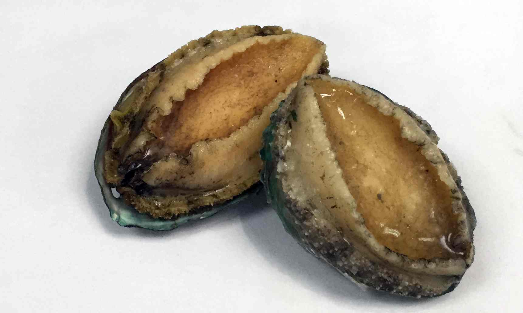The Abalone is a type of marine snail animal. The age of an Abalone can be found by counting the number of rings in its shell using a microscope, which is a laborious task. This collected dataset allows us to attempt to predict the age (rings) of the Abalone without actually counting the rings. Features measured include length, width and weight of the abalone as well as its sex.

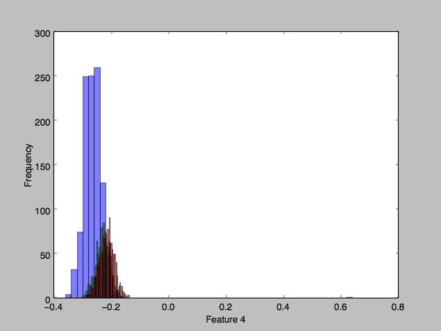
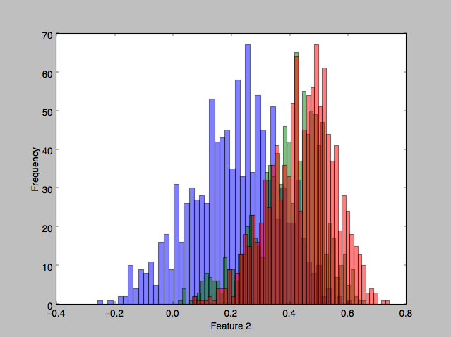
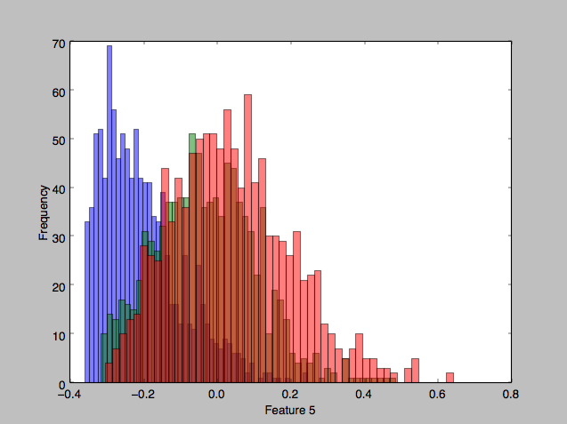
This dataset consists of 4177 samples with an age distribution as shown here. I set aside 25% of this dataset for test, and trained on the remaining 75%. The data was partitioned into 3 roughly equally sized classes for the classification task: (1) Ages 1-8, (2) ages 9-10, (3) 11-29.

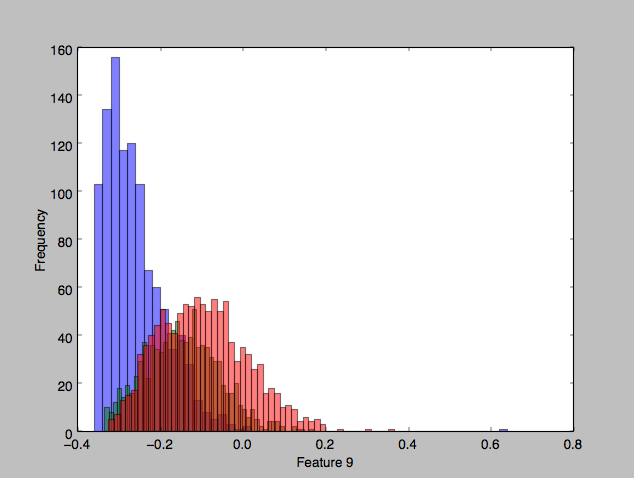
Looking at some of the features’ histograms, it does appear than there is considerable overlap in the classes, especially in the second two classes (red and green).

 

Bayes plug-in classifier

With the Gaussian Bayes classifier, the test accuracy obtained is around 61.2% which is not too much worse than the other classifiers I tried later (nor compared to the results reported by the original investigators of the dataset.) Although, we should note that pure guessing would give us a 33% test accuracy, so a ~60% accuracy isn’t all that much to get excited about.

Implementation notes

• Categorical features (e.g. sex = Male/Female/Infant): I initially considered simply encoding these as 0/1/2, but that would be wrong because these categories don’t actually have a linear relationship. The right way is to have a boolean feature for each.
• Singular matrices: However, creating 3 separate boolean features resulted in problems running the Bayes classifier. The determinant value for calculating the Gaussians ended up very close to zero (10^-43 i.e., the covariance matrix was non-invertible / singular. This makes sense, because knowing the values of two of the features completely determines the value of the third feature, i.e., the columns are not mutually independent. Dropping one of the three columns fixed the problem.
• Further work: Perhaps I could fine-tune the threshold values to use for the different class assignments instead of simply weighting them all equally. Say, using ROC curves. I have yet to explore this option.

Naive Bayes classifier

With the Naive Gaussian Bayes classifier, I got a test accuracy of 58.7% which is predictably worse than the full Gaussian classifier above, but not much worse.

Perceptron

Running the perceptron algorithm on the Abalone dataset gave me a 54.9% test accuracy. Considering that the data doesn’t have a fully separating hyperplane (and in fact has a lot of overlap), I’m surprised that the perceptrons performance wasn’t way worse.

Implementation notes

• Multiple classes: I had to extend the perceptron algorithm to work with multiple classes, which meant training a classifier (finding a hyperplane) for each class.  However, since the classes are linearly related (and since our hyperplanes cannot curve) it becomes impossible to classify any of the “middle” classes; these would be better handled by two bounding hyperplanes.
  Eventually, instead of setting the perceptrons to be “this class vs. the rest” classifiers, I got the perceptrons to search for the hyperplanes between adjacent classes, and assigned each data point to an appropriate class based on which side of each hyperplane it fell on.
  Specifically, I assigned the data point to the class corresponding to the first hyperplane whose dot product with the data point was negative.
• Number of iterations: As expected, the Perceptron doesn’t converge fully but running it for a large enough number of iterations seems to give decent results. I got the (modestly) best results around 8000 iterations, and interestingly the test accuracy seemed to slowly drop off beyond that.
• Individual vs Overall accuracy: Despite each of the (two) hyperplanes performing quite good (at 70-80% accuracy individually) their combined classification accuracy is noticeably less (54%). This is a result of the fact that the error rate is cumulative. Attempting to subdivide a class into two classes and to correctly classify its data-points across these two smaller classes can only increase the error rate.

Logistic Regression

I implemented the gradient descent Logistic Regression classifier (for multiple classes) with Regularization, and was able to get a 64.7% test accuracy, which is the best of the lot I’ve attempted so far.

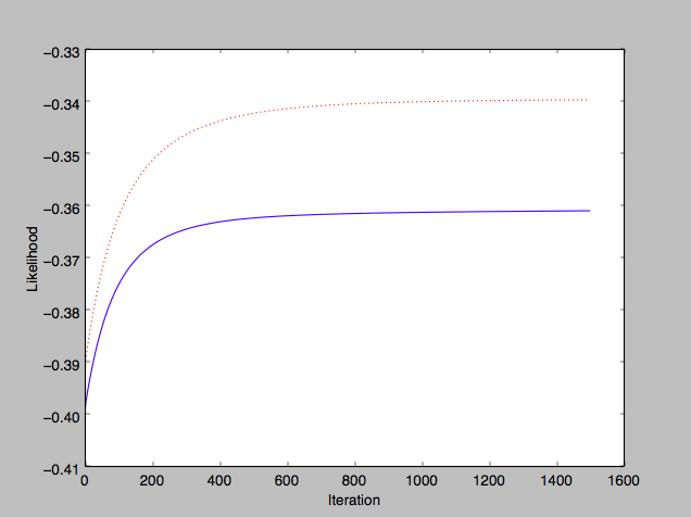
Plotting the model’s training and test set average likelihoods vs number of iterations run, I see a good improvement in training (blue) and test (red) accuracy:

 

 

Implementation notes

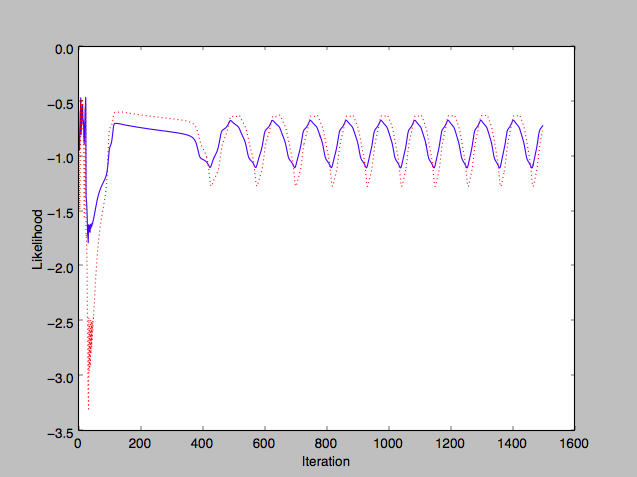
• Learning rate: The quality of the resulting Logistic Regression model seems to depend a lot on the learning rate as well as the regularization constant. Too high of a learning rate can lead to very unpredictable movement:
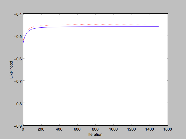
• Test likelihood: Initially when I tried plotting the test results in the above graph, I realized I was comparing likelihood of training set vs accuracy of test set. I thereafter reworked the graph calculation to plot the (average) computed likelihood of the test predictions as well.
• Regularization and weights: In order to understand the effect of regularization on the values of the weight vector w, I tried to compare w across different regularization runs. However, the differences in w varied quite randomly, and this is perhaps due to correlations amongst the features/axes in the dataset.
• Bias: I ran the Logistic Regression algorithm on the earlier wdbc dataset, which is known to have a separating hyperplane. However, it was difficult to find this hyperplane using Logistic Regression especially when I used regularization — and this makes sense because regularization introduces bias. Training dataset will perform worse with regularization than without.
• Feature expansion: In an attempt to increase test accuracy by introducing polynomial elements into the feature set, I manually tried a few ideas, e.g. the product of length, width and height (i.e. volume), and the square of the length. However, I found that the accuracy barely improved, and sometimes in fact got worse.
  I also tried reintroducing the “Infant” boolean column (which I had taken out for the Gaussian Bayes classifier) but there was no effect on accuracy
• Further work: Ideas to try out:
  • I could try dampening the learning rate of the gradient descent, to perhaps make faster progress in the algorithm.
  • Better / automated feature selection.

k Nearest Neighbor

I implemented the straightforward k-nearest neighbor algorithm to try on the Abalone dataset, and the test accuracy I got was just around 64-66% which seems to reflect the amount of overlap in the data. There was no clear value of k to use either, since it depended a lot on the portion of the data I used for training. I found that values of k around 20-25 seemed slightly better performing than others.

Implementation notes

• Algorithm performance: With k-NN there is no real ‘training’ beyond storing the training set in memory. The bulk of the work occurs during classification, and since this involves individually finding for each test data point the closest k neighbors from all the available training data points, this ends up being a rather slow algorithm. I found it hard to vectorize the algorithm in a way that would speed things up.
• Normalization: is very important here, since we want to treat every feature as equally important.
• l_p distance: Instead of using only the Euclidean l_2 distance, I tried running the algorithm with varying types of distance measures. I found that p=2 performed quite well enough, although p=1.5 sometimes performed better.
• Density: What does it mean for the density of one class to be much higher than the other? E.g. what if class A has way more training samples than class B, wouldn’t that distort the k-NN? My answer to this is that it wouldn’t, because the higher density merely indicates a higher probability (prior probability) of occurrence of class A.
• Further work:
  • Curse of dimensionality: kNN suffers from the problem of sparseness when too many features/axes are in play. Feature selection could really help here.
  •  Soft k-NN: is a version of k_NN in which the “k” is not a fixed boundary. Instead, all the training data points are taken into accounted, but weighted by proximity to the test data point.

 

---

Update: March 23, 2018

Support Vector Machine

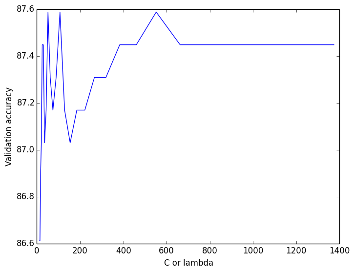
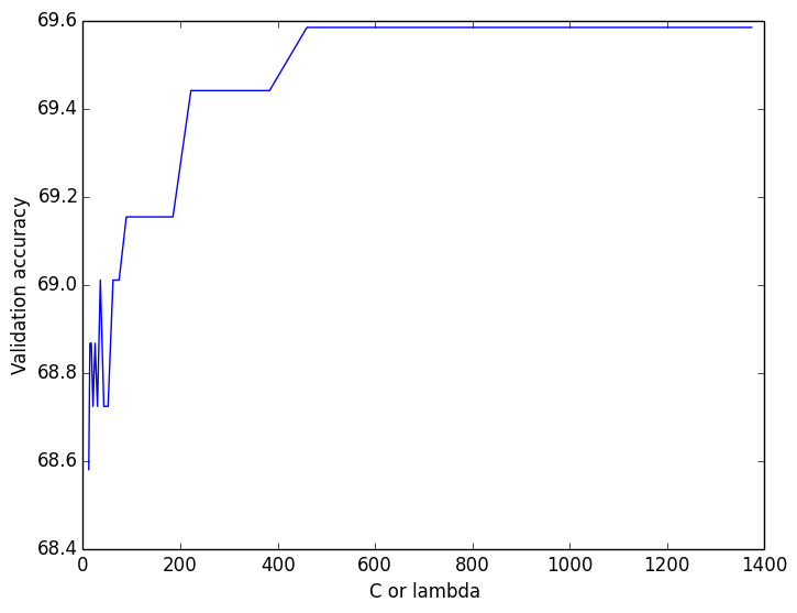
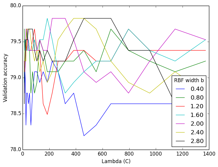
I implemented the Support Vector Machine algorithm with the help of CVXOPT (a QP problem solver) and also implemented per-class cross-validation to identify good model parameters to use for the Abalone dataset. Details are in my SVM implementation notes

The hard-margin linear SVM classifier predictably gave very poor results (despite using one-vs-one multi-class classification) because of the overlap between the classes.

The soft-margin RBF-kernelized SVM classifier gave much better results. Cross validation determined ideal set of parameters (on the validation set), which gave me an overall accuracy (on the test set) of 67.4% which is the highest I’ve obtained so far on the Abalone dataset.

 

 

 

A soft-margin linear SVM using one-vs-one classification also performed pretty well. I ran cross-validation across lambda:

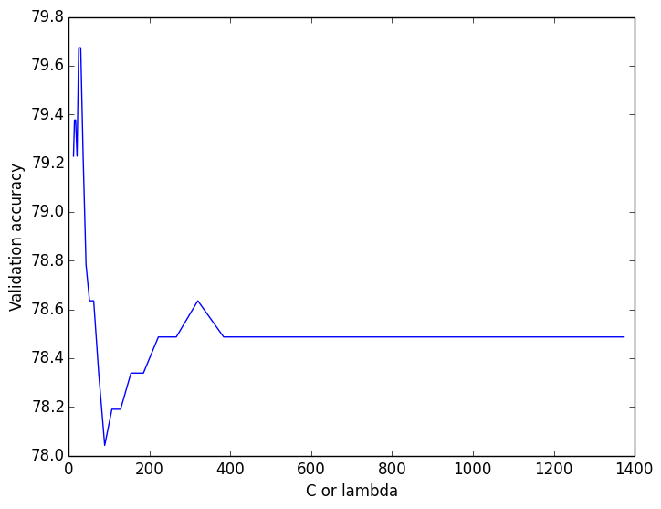
… and picking the good lambda values gave me an overall test accuracy of 65.9%.

A soft-margin RBF-kernelized SVM using one-vs-one classification performed nearly as well as the equivalent one-vs-all classification, with a test-accuracy of 66.9%. Although, picking good parameters from the validation results was a little less obvious.